Chapter 3 More Linear Programming Models
3.1 Types of LP Models
In this chapter, we will examine a range of classic applications of linear programs. These applications will give ideas for how to model a variety of situations. In each case, try to follow along with the application.
3.2 The Algebraic Model
In the previous chapter, we examined situations with only a few products and constraints. In general, most companies have many more products and we won’t be wanting to name each variable explicitly and uniquely. We refer to this type of model as an explicit linear program. Instead, we use sets of products and resources.
We could also reframe the model more algebraically. Let’s use subscripts to differentiate between products and resources. We can define to i=1 to represent Ants, i=2 to represent Bats, and i=3 to represent Cats. Similarly, j=1 represents machining, j=2, represents assembly, etc.
Now, let’s move on to defining the data. Let’s define the amount to produce of each product, i, as \(x_i\) and resource j consumed by product i as \(R_{i,j}\). The available resource j is then \(A_j\). The profit per product i is then \(P_i\). The LP can now be rewritten as shown below with the three products and four constraints.
\[ \begin{split} \begin{aligned} \text{Max } & \sum_{i=1}^3 P_i x_i \\ \text{s.t.: } & \sum_{i=1}^3 R_{i,j}x_i \leq A_j, \; j=1, 2, 3, 4\\ & x_1, \; x_2, \;x_3 \geq 0 \end{aligned} \end{split} \]
We could further generalize this by eliminating the hard coding of the number of products and resource constraints. Instead we define the number of products and resources as NProd and NResources respectively.
Let’s introduce a very convenient shorthand symbol, \(\forall\), is read as “for all.” It can be interpreted to mean “repeat by substituting for all possible values of this subscript.” In the constraint, it means to repeat the constraint line with \(j=1\), again with \(j=2\), and so on for as many values of j as make sense in the model.
We also will use it in the non-negativity constraint to avoid having to list out every variable, x_1, x_2, etc. In other words, given that i is used consistently for the three products, then \(x_i \geq 0 \; \forall \; i\) is equivalent to \(x_i \geq 0 \;,i=1,2,3\) or even \(x_1 \geq 0, \; x_2 \geq 0, \; x_3 \geq 0\).
The payoff is modest when there are 3 products and 4 constraints but when there are hundreds of products and thousands of constraint, the benefit is tremendous. Furthermore, the generalized, algebraic model doesn’t change when a new product is added or one is discontinued, it is only a change of data that is fed into the model. The result is that the \(\forall\) symbol can simplify the description of complex models when index ranges are clear.
We can then rewrite the previous formulation as the following, more general formulation.
\[ \begin{split} \begin{aligned} \text{Max:} & \sum_{i=1}^{NProd} P_i x_i \\ \text{subject to } & \sum_{i=1}^{NProd} R_{i,j}x_i \leq A_j \; \forall \; j\\ & x_i \geq 0 \; \forall \; i \end{aligned} \end{split} \]
It is even more important to clearly and precisely define the meanings of variable and data element in an algebraic model than in an explicit model.
3.2.1 Tips and Conventions for Algebraic Models
Learning how to read and write mathematical models is an important skill. In this section we will provide a quick overview. More information is provided in Appendix B.
Another good practice is to use a mnemonic to help suggest the meaning of data. That is why I chose “R” for Resource, “P” for Profit, and “A” for Available resources.
A helpful convention is to use capital letters for data and lower case letters for variables. Some people will swap this around and use capital letters for variables and lower case letters for data - it doesn’t matter as long as a model is consistent. It gives a quick visual cue for the reader as to whether each item is a variable or constraint.
More complex models often run out of letters that make sense.
A common approach in these models is to use a superscript.
For example, perhaps labor cost for each worker, w, could have different values for both normal and overtime rates.
Rather than separate data terms for such closely related concepts, we might denote regular hourly labor cost for worker w as \(C^R_w\) and for overtime as \(C^O_w\). Another option is to use a Greek letter such as \(\theta\). We’ll see a few Greek letters used in chapter 5.
Again, this highlights why it is very important to clearly define all the data and variables used in the model. Think of it as building a language for describing the particular model. It is frequently an iterative process that it is updated as the model is refined and developed. Frequently a definitions section will warrant its own section or subsection and should precede the formulation.
3.2.2 Building the Generalized Model in R
3.2.2.1 Preparing the Data
The concise, algebraic representation can be easily scaled to any number of products and resources. I’ll expand the names of data slightly for making the R code more readable but this is meant to be consistent with the above formulation.
| Prod1 | Prod2 | Prod3 | Prod4 | |
|---|---|---|---|---|
| Profit | 7 | 10 | 5 | 24 |
Let’s implement a four product model requiring varying levels of five limited resources. We will start our implementation by creating the appropriate data structures in R.
NProd <- 4
NResources <- 5
ProdNames <- lapply(list(rep("Prod",NProd)),paste0,1:NProd)
                 # Product names: Prod1, Prod2, ...
Profit <- matrix(c(20, 14, 3, 16),
              ncol=NProd,dimnames=c("Profit",ProdNames))
ResNames<- lapply(list(rep("Res",NResources)),
                  paste0,1:NResources)
                 # Resource names: Res1, Res2, ...
Resources <- matrix(c( 1, 3, 2, 3, 2, 3, 4, 3, 5, 7,
                       2, 2, 1, 2, 2, 2, 2, 2, 4, 6),
              ncol=NProd,
              dimnames=c(ResNames,ProdNames))
Available <- matrix(c(800, 900, 480, 1200, 500),
              ncol=1,dimnames=c(ResNames,"Available"))
This should match the data that we hard coded into the R linear programming model in the previous chapter.
Similarly, we can display the resources used by each product and the amount of each resource available alongside each other.
Combined <- cbind(Resources, Available)
kbl(Combined, booktabs=T,
    caption="Resources Used by Each Product and Amount Available") |>
kable_styling(latex_options = "hold_position")| Prod1 | Prod2 | Prod3 | Prod4 | Available | |
|---|---|---|---|---|---|
| Res1 | 1 | 3 | 2 | 2 | 800 |
| Res2 | 3 | 4 | 2 | 2 | 900 |
| Res3 | 2 | 3 | 1 | 2 | 480 |
| Res4 | 3 | 5 | 2 | 4 | 1200 |
| Res5 | 2 | 7 | 2 | 6 | 500 |
We have used the cbind function to do a column binding of the data.
In this way the representation is more visually intuitive.
To ensure that we know how to access the data, if we want to see how the amount of the first resource used by the second product, you can enter Resources[1,2] in R Studio’s console which is then evaluated as 3.
Using inline code is a great feature of RMarkdown. In the text of your RMarkdown, anything enclosed by a pair of single tick marks will be shown as a code chunk. If it starts with the letter r, it will be passed instead to R for evaluation. This allows for discussing results in a reproducible manner.
For example, rather than discussing a result giving a value of 42.00 in the text and a later rerun of the analysis has an updated table of results showing the result to be 42.42, by using inline code evaluation, it will always show the up to date result.
Now, let’s begin building our optimization model.
3.2.2.2 Implementing the Model
First, we’ll start by loading the packages that we are using. I’ll typically do this as at the beginning of an RMarkdown document but for demonstration purposes, I’ll put it here at the beginning of our model implementation. It is important to note that when knitting an RMarkdown document, it will run as a fresh environment without having items in memory from your environment and packages loaded. When you run all code chunks, it will retain the currently loaded packages.
suppressPackageStartupMessages(library (dplyr, quietly = TRUE))
suppressPackageStartupMessages(library (ROI, quietly = TRUE))
library (ROI.plugin.glpk, quietly = TRUE)
library (ompr, quietly = TRUE)
library (ompr.roi, quietly = TRUE)
We will continue with the code to build the model in a generic format. Note that in my ompr model, I generally like to give each linear programming variable in ompr a V prefix to differentiate it from a regular R data object that might exist elsewhere in my R environment. Conflicts between R objects and ompr variables are a common problem for modelers and this helps to avoid the problem, assuming that you don’t have a lot of other R objects that start with V. For more discussion about this issue and other common problems that are particularly common in optimization modeling using R, see Appendix C.
prodmodel <- MIPModel()                          |>
  add_variable (Vx[i], i=1:NProd,
                type="continuous", lb=0)         |>
  set_objective (sum_expr(Profit[i] * Vx[i],
                          i=1:NProd ), "max")    |>
  add_constraint (sum_expr(Resources[j,i]*Vx[i],
                           i=1:NProd)
                  <= Available[j],
                  j=1:NResources)                |>

  solve_model(with_ROI(solver = "glpk"))

prodmodel
## Status: optimal
## Objective value: 48003.2.3 Examining the Results
Displaying the object of prodmodel only shows a simple summary of the results of the analysis.
It indicates whether the model was solved to optimality (and it was!) and the objective function value (profit).
This is useful to know but we are really interested in how to generate this profit.
To do this, we need to extract the values of the variables.
results.products <- matrix (rep(-1.0,NProd),
                            nrow = NProd, ncol=1,
                            dimnames=c(ProdNames,c("x")))
temp <- get_solution (prodmodel, Vx[i])
   # Extracts optimal values of variables
results.products <- t(temp [,3] )
   #Extracts third column
results.products <- matrix (results.products,
                            nrow = 1, ncol=NProd,
                            dimnames=c(c("x"),ProdNames))
                            # Resizes and renames
kbl(format(head(results.products),digits=4), booktabs=T,
    caption="Optimal Production Plan") |>
kable_styling(latex_options = "hold_position")| Prod1 | Prod2 | Prod3 | Prod4 | |
|---|---|---|---|---|
| x | 240 | 0 | 0 | 0 |
The table displays the optimal production plan.
Let’s examine how the resources are consumed.
To do this, we can multiply the amount of each product by the amount of each resource used for that product.
For the first product, this would be a term by term sum of each product resulting in 240 which is less than 800.
We can do this manually for each product.
Another approach is to use the command, Resources[1,]%*%t(results.products).
This command will take the first row of the Resources matrix and multiplies it by the vector of results.
Note how we used both an inline r expression and an inline executable r code chunk. Inline code chunks can be inserted into text by using a single tick at the beginning and end of the chunk instead of the triple tick mark for regular code chunks. Also, the inline r code chunk starts with the letter r to indicate that it is an r command to evaluate. A common use for this might be to show the results of an earlier analysis.
One thing to note is that the first row of Resources is by definition a row vector and result.products is also a row vector.
What we want to do is do a row vector multiplied by a column vector.
In order to do this, we need to convert the row vector of results into a column vector.
This is done by doing a transpose which changes the row to a column.
This is done often enough that the actual function in R is just a single letter, t.
We can go one further step now and multiply the matrix of resources by the column vector of production.
results.Resources <- Resources[]%*%t(results.products)
# Multiply matrix of resources by amount of products produced
ResourceSlacks <- cbind (results.Resources,
                         Available,
                         Available-results.Resources)
colnames(ResourceSlacks)<-c("Used", "Available", "Slack")
kbl(format(head(ResourceSlacks),digits=4), booktabs=T,
    caption="Resources Used in Optimal Solution") |>
kable_styling(latex_options = "hold_position")| Used | Available | Slack | |
|---|---|---|---|
| Res1 | 240 | 800 | 560 |
| Res2 | 720 | 900 | 180 |
| Res3 | 480 | 480 | 0 |
| Res4 | 720 | 1200 | 480 |
| Res5 | 480 | 500 | 20 |
This section covered a lot of concepts including defining the data, setting names, using indices in ompr, building a generalized ompr model, extracting decision variable values, and calculating constraint right hand sides. If you find this a little uncomfortable, try doing some experimenting with the model. It may take some experimenting to get familiar and comfortable with this.
3.2.4 Changing the Model
Let’s modify the above model. We can do this by simply changing the data that we pass into the model and rebuilding the model.
Let’s change the number of sensors required for an Ant to 5. Recall that this is the first product and the fourth resource. This is how we can change the value.
Resources[4,1] <- 5
# Set value of the 4th row, 1st column to 5
# In our example, this is the number of sensors needed per Ant
Now we will rebuild the the optimization model. Note that simply changing the data does not change the model.
prodmodel <- MIPModel() |>
  add_variable (Vx[i], i=1:NProd,
                type="continuous", lb=0)       |>
  set_objective (sum_expr(Profit[i] * Vx[i] ,
                          i=1:NProd ), "max")  |>
  add_constraint (sum_expr(Resources[j,i]*Vx[i],
                           i=1:NProd)
                  # Left hand side of constraint
                  <= Available[j],
                  # Inequality and Right side of constraint
                  j=1:NResources)              |>
                  # Repeat for each resource, j.
  solve_model(with_ROI(solver = "glpk"))

prodmodel
## Status: optimal
## Objective value: 4800We can see that the objective function has changed.
results.products <- matrix (rep(-1.0,NProd),
                            nrow = NProd,
                            ncol=1,
                            dimnames=c(ProdNames,c("x")))
temp <- get_solution (prodmodel, Vx[i]) # Extracts optimal values of variables
results.products <- t(temp [,3] )       # Extracts third column
results.products <- matrix (results.products,
                            nrow = 1,
                            ncol=NProd,
                            dimnames=c(c("x"),ProdNames))
   # Resizes and renames
kbl(results.products, booktabs=T,
    caption="Revised Optimal Production Plan")  |>
kable_styling(latex_options = "hold_position")| Prod1 | Prod2 | Prod3 | Prod4 | |
|---|---|---|---|---|
| x | 240 | 0 | 0 | 0 |
The production plan has significantly changed.
3.3 Common Linear Programming Applications
3.3.1 Blending Problems
Specific blend limitations arise in many situations. Recall from our three variable case in Chapter 2 that the vast majority of drones produced were Cat models. Let’s assume that we can’t have more than 40% of total production made up of Cats. Let’s start by building our original three variable model. In our original case, this would be expressed as the following.
\[ \begin{split} \begin{aligned} \text{Max } & 7\cdot Ants +12 \cdot Bats +5\cdot Cats \\ \text{s.t.:} & \\ & 1\cdot Ants + 4\cdot Bats +2\cdot Cats \leq 800 \\ & 3\cdot Ants + 6\cdot Bats +2\cdot Cats \leq 900 \\ & 2\cdot Ants + 2\cdot Bats +1\cdot Cats \leq 480 \\ & 2\cdot Ants + 10\cdot Bats +2\cdot Cats \leq 1200 \\ & Ants, \; Bats, \; Cats \geq 0 \end{aligned} \end{split} \]
Let’s rebuild our three variable implementation and review the results to see if it is violates our blending requirement.
model1 <- MIPModel()                              |>
  add_variable(Ants, type = "continuous", lb = 0) |>
  add_variable(Bats, type = "continuous", lb = 0) |>
  add_variable(Cats, type = "continuous", lb = 0) |>

  set_objective(7*Ants + 12*Bats + 5*Cats,"max")  |>

  add_constraint(1*Ants + 4*Bats + 2*Cats<=800)   |> # machining
  add_constraint(3*Ants + 6*Bats + 2*Cats<=900)   |> # assembly
  add_constraint(2*Ants + 2*Bats + 1*Cats<=480)   |> # testing
  add_constraint(2*Ants + 10*Bats + 2*Cats<=1200)    # sensors

res3base <-  solve_model(model1, with_ROI(solver="glpk"))

xants <- get_solution (res3base, Ants)
xbats <- get_solution (res3base, Bats)
xcats <- get_solution (res3base, Cats)
base_case_res           <- cbind(xants,xbats,xcats)
rownames (base_case_res) <- "Amount"
colnames (base_case_res) <- c("Ants","Bats","Cats")kbl(base_case_res, booktabs=T,
caption="Production Plan for Base Case") |>
kable_styling(latex_options = "hold_position")| Ants | Bats | Cats | |
|---|---|---|---|
| Amount | 50 | 0 | 375 |
These results clearly violate the required production mix for Cats. Let’s now work on adding the constraint that Cats can’t make up more than 40% of the total production.
\[\frac{Cats}{Ants+Bats+Cats} \leq 0.4\]
Alas, this is not a linear function since we are dividing a variable by a function of variables so we need to clear the denominator. For demonstration purposes, we will write out each step.
\[Cats \leq 0.4 \cdot (Ants+Bats+Cats)\]
We like to get all the variables on the left side so let’s move them over.
\[Cats - 0.4 \cdot Ants-0.4 \cdot Bats-0.4 \cdot Cats \leq 0\]
Let’s simplify this a little, which gives us the following:
\[-0.4 \cdot Ants-0.4 \cdot Bats+0.6 \cdot Cats \leq 0\]
Now we can just this to the original formulation. The result is the following formulation.
\[ \begin{split} \begin{aligned} \text{Max } & 7\cdot Ants +12 \cdot Bats +5\cdot Cats \\ \text{s.t.:} & \\ & 1\cdot Ants + 4\cdot Bats +2\cdot Cats \leq 800 \\ & 3\cdot Ants + 6\cdot Bats +2\cdot Cats \leq 900 \\ & 2\cdot Ants + 2\cdot Bats +1\cdot Cats \leq 480 \\ & 2\cdot Ants + 10\cdot Bats +2\cdot Cats \leq 1200 \\ & \textcolor{red}{-0.4 \cdot Ants-0.4 \cdot Bats +0.6 \cdot Cats \leq 0}\\ & Ants, \; Bats, \; Cats \geq 0 \end{aligned} \end{split} \]
We can simply add a constraint to an existing ompr model of our 3 variable base case and then solve again.
ModelBlending<- add_constraint(model1,
                -0.4*Ants -0.4*Bats +0.6*Cats <= 0)
resBlending<- solve_model(ModelBlending,
with_ROI(solver = "glpk"))blendres<-cbind(get_solution (resBlending, Ants),
get_solution (resBlending, Bats),
get_solution (resBlending, Cats))Okay, now let’s put both side by side in a table to show the results.
rownames(base_case_res)<-"Base Model"
rownames(blendres)<-"with Constraint"
comparative <- rbind(base_case_res,round(blendres, 2))
colnames (comparative) <- c("Ants","Bats","Cats")
kbl(comparative, booktabs=T,
    caption =
      "Compare Baseline and Production Plan with Blending Constraint")|>
kable_styling(latex_options = "hold_position")| Ants | Bats | Cats | |
|---|---|---|---|
| Base Model | 50 | 0 | 375 |
| with Constraint | 140 | 40 | 120 |
The table clearly shows that the blending constraint had a major impact on our product mix.
3.4 Allocation Models
An allocation model divides resources and assigns them to competing activities. Typically it has a maximization objective with less than or equal to constraints. Note that our production planning problem from Chapter 2 is an allocation model.
\[ \begin{split} \begin{aligned} \text{Max: } & \sum_{i=1}^3 P_i x_i &\text{[Maximize Profit]}\\ \text{s.t. } & \sum_{i=1}^3 R_{i,j} x_i \leq A_j \; \forall \; j &\text{[Resource Limits]}\\ & x_i \geq 0 \; \forall \; i \end{aligned} \end{split} \]
3.4.1 Covering Models
A covering model combines resources and coordinates activities. A classic covering application would be what mix of ingredients “covers” the requirements at the lowest possible cost. Typically it has a minimization objective function and greater than or equal to constraints.
\[ \begin{split} \begin{aligned} \text{Min:} & \sum_{i=1}^3 C_i x_i &\text{[Minimize Cost]}\\ \text{S.t.} & \sum_{i=1}^3 A_{i,j}x_i \geq R_j \; \forall \; j &\text{[Meet Requirements]}\\ & x_i \geq 0 \; \forall \; i \end{aligned} \end{split} \]
Consider the case of Trevor’s Trail Mix Company. Trevor creates a variety of custom trail mixes for health food fans. He can use a variety of ingredients displayed in following table.
| Characteristic | Mix1 | Mix2 | Mix3 | Mix4 | Min Req. |
|---|---|---|---|---|---|
| Cost | $20 | $14 | $3 | $16 | |
| Calcium | 6 | 2 | 1 | 4 | 1440 |
| Protein | 8 | 6 | 1 | 8 | 1440 |
| Carbohydrate | 6 | 4 | 1 | 25 | 2000 |
| Calories | 7 | 10 | 2 | 12 | 1000 |
Let’s go ahead and build a model in the same way as we had done earlier for production planning.
NMix <- 4
NCharacteristic <- 4
MixNames <- lapply(list(rep("Mix",NMix)),paste0,1:NMix)
                 # Mix names: Mix1, Mix2, ...
CharNames <-lapply(list(rep("Char",NCharacteristic)),
                   paste0,1:NCharacteristic)
                 # Characteristics of each mix
Cost <- matrix(c(20, 14, 3, 16),
              ncol=NMix,dimnames=c("Cost",MixNames))
MixChar <- matrix(c( 6, 8, 6, 7,
                     2, 6, 4, 10,
                     1, 1, 1, 2,
                     4, 8, 25, 12),
              ncol=4, dimnames=c(CharNames,MixNames))
CharMin <- matrix(c(1440, 1440, 2000, 1000),
              ncol=1,dimnames=c(CharNames,"Minimum"))
TTMix <-cbind(MixChar,CharMin)
kbl(TTMix, booktabs=T,
caption="Data for Trevor Trail Mix Company") |>
kable_styling(latex_options = "hold_position")| Mix1 | Mix2 | Mix3 | Mix4 | Minimum | |
|---|---|---|---|---|---|
| Char1 | 6 | 2 | 1 | 4 | 1440 |
| Char2 | 8 | 6 | 1 | 8 | 1440 |
| Char3 | 6 | 4 | 1 | 25 | 2000 |
| Char4 | 7 | 10 | 2 | 12 | 1000 |
Hint: You might need to add a total amount to make! Modify the numbers until it runs.
Now let’s build our model.
trailmixmodel <- MIPModel()                             |>
 add_variable(Vx[i],i=1:NMix,type="continuous",lb=0)    |>
 set_objective(sum_expr(Cost[i]*Vx[i],i=1:NMix ),"min") |>
 add_constraint(sum_expr(MixChar[j,i]*Vx[i],i=1:NMix)  # LHS
                  >= CharMin[j],          # Inequality and RHS
                  j=1:NCharacteristic)    # Repeat for each resource

results.trailmix <- solve_model(trailmixmodel,
                                with_ROI(solver = "glpk"))

results.trailmix
## Status: optimal
## Objective value: 4426.667xvalue <- t(get_solution(results.trailmix, Vx[i])[,3])We’ll leave it to the reader to clean up the output of results.
Another classic example of a covering problem is a staff scheduling problem. In this case, a manager is trying to assign workers to cover the required demands throughout the day, week, or month.
3.4.2 Transportation Models
A transportation model is typically for getting material from one place to another at the lowest possible costs. It has sets of source points or nodes as well as ending or destination nodes. The decision variables are the amount to send on each route. Constraints are typically based on supply from the source nodes and capacity at the destination nodes.
This naturally lends itself to potential network diagrams such as the one to the right. In this case we have three warehouses (or supply points) in Minnesota (MN), Pennsylvania (PA), and Wyoming (WY), each with a supply shown to the left. On the right side, we have four customer or demand nodes: Atlanta (ATL), Boston (Bos), Chicago (Chi), and Denver (Den) with their maximum demand shown to the right of the node. We also have arcs connecting every supply node to every demand node, each labeled with a corresponding cost per unit to transport an item along that arc. The goal is to get as much shipped as possible at the lowest possible cost.
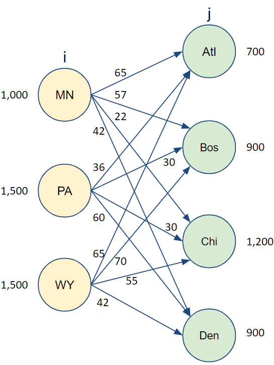
FIGURE 3.1: Transporation Example
Let’s start to model this now. We want to define the decision variables, in this case, \(x_{i,j}\) is the amount of product to ship from node i to node j.
Let’s also define the data available. The cost per unit to ship from node i to node j is \(C_{i,j}\).
The supply available from each supply node is \(S_i\) and the maximum demand that can be accommodate from each destination node is \(D_j\).
In this formulation we need to make sure that we don’t ship out more than the capacity of each supply node.
Similarly, we need to ensure that we don’t take in more than demand capacity at any destination.
\[ \begin{split} \begin{aligned} \text{Min } & \sum_{i} \sum_{j} C_{i,j} x_{i,j} \\ \text{s.t. } & \sum_{i} x_{i,j} \leq D_j \; \forall \; j&\text{[Demand Limits]}\\ & \sum_{j} x_{i,j} \leq S_i \; \forall \; i&\text{[Supply Limits]}\\ & x_{i,j} \geq 0 \; \forall \; i,j \end{aligned} \end{split} \]
If we simply run this model, as is, the minimum cost plan would be to just do nothing! The cost would be zero. In reality, even though we are focused on costs in this application, there is an implied revenue and therefore profit (we hope!) that we aren’t directly modeling. We are likely to instead be wanting to ship all of the product that we can at the lowest possible cost. More precisely, what we want to do is instead determine if the problem is supply limited or demand limited. This is a simple matter of comparing the net demand vs. the net supply and making sure that the lesser is satisfied completely.
| If… | Then Situation is: | Source Constraints | Demand Constraints |
|---|---|---|---|
| \(\sum_{i} S_i < \sum_{j} D_j\) | Supply Constrained | \(\sum_{j} x_{i,j} = S_i\) | \(\sum_{i} x_{i,j} \leq D_j\) |
| \(\sum_{i} S_i > \sum_{j} D_j\) | Demand Constrained | \(\sum_{j} x_{i,j} \leq S_i\) | \(\sum_{i} x_{i,j} = D_j\) |
| \(\sum_{i} S_i = \sum_{j} D_j\) | Balanced | \(\sum_{j} x_{i,j} = S_i\) | \(\sum_{i} x_{i,j} = D_j\) |
In the balanced situation, either source or demand constraints can be equalities.
Similarly, if we try to use equality constraints for both the supply and demand nodes but the supply and demand are not balanced, the LP will not be feasible.
In ompr, a double subscripted non-negative variable, \(x_{i,j}\) can be defined easily as the following:
add_variable(x[i, j], type = "continuous", i = 1:10, j = 1:10, lb=0). Let’s show how to set up a basic implementation of the transportation problem in ompr. This demonstrates the use of double subscripted variables. Also, it should be customized for a particular application of being demand or supply constrained but it will give a good running head start.
NSupply <- 3   # 3 Supply nodes
NDest   <- 4   # 4 Destination nodes
snames <- list("MN", "PA", "WY")
dnames <- list("Atl", "Bos", "Chi", "Den")
Cost <- matrix (c(65, 36, 65, 57, 30, 70,
                  22, 30, 55, 42, 60, 42),
                nrow = NSupply,
                dimnames =list(snames,dnames))
S <- c(1000, 1500, 1500)

D <- c(700,  900, 1200, 900)
At this point, it may be a good idea to look at the arcs and see if you can expect which routes are likely to be heavily used and which are likely to be unused. You can also do this by looking at the matrix of transportation costs.
| Atl | Bos | Chi | Den | |
|---|---|---|---|---|
| MN | 65 | 57 | 22 | 42 |
| PA | 36 | 30 | 30 | 60 |
| WY | 65 | 70 | 55 | 42 |
Now, let’s move on to implementing the model.
transportationmodel <- MIPModel()             |>
 add_variable(Vx[i, j], type = "continuous",
               i = 1:NSupply,
               j = 1:NDest, lb=0)             |>
 set_objective (sum_expr(Cost[i,j] * Vx[i,j] ,
                          i=1:NSupply,
                          j=1:NDest ), "min") |>
 add_constraint (sum_expr(Vx[i,j], i=1:NSupply)
                >= D[j],
                j=1:NDest)|>
 add_constraint (sum_expr(Vx[i,j], j=1:NDest)
                <= S[i],
                i=1:NSupply)

res.transp <-solve_model(
  transportationmodel, with_ROI(solver ="glpk"))
Let’s confirm that our model solved correctly.
res.transp$status## [1] "optimal"Since it was solved to optimality, the optimal objective function value is meaningful and again we can use an inline code chunk of R to extract this value 1.259^{5}. The actual decision variable values of the solution are more interesting though. Let’s first prepare these results by extracting them from the solution object and then applying our names to them.
Transp <- matrix(res.transp$solution,
                nrow = NSupply,
                dimnames =list(snames,dnames))
Now we can display the table of optimal transportation decisions from supply points to destinations cleanly.
| Atl | Bos | Chi | Den | |
|---|---|---|---|---|
| MN | 0 | 0 | 1000 | 0 |
| PA | 600 | 900 | 0 | 0 |
| WY | 100 | 0 | 200 | 900 |
3.4.3 Transshipment Models
A generalization of the transportation model is that of transshipment where some nodes are intermediate nodes that are neither pure sources or destinations but can have both inflow and outflow. We could extend our previous example with factories in Vietnam and Thailand. Note that the facilities in the middle (Minnesota, Pennsylvania, and Wyoming) are better described as distribution centers rather than warehouses.
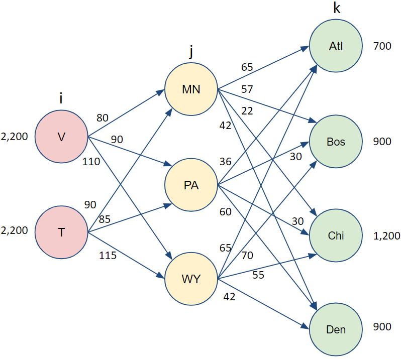
FIGURE 3.2: Transshipment Application.
In this case, the standard convention might be to work from left to right and index the set of factories by i, the set of distribution centers by j and the set of customers by k. We might also use \(x_{i,j}\) to be the amount to ship from factory i to distribution center j and \(y_{j,k}\) to be the amount to ship from distribution center j to customer k.
A common characteristic of this kind of problem is then that the inflow at each distribution center must equal the outflow. This means that for Minnesota, \((j=1)\), we would would have a relationship of the following.
\[x_{1,1}+x_{2,1}=y_{1,1}+y_{1,2}+y_{1,3}+y_{1,4}\]
This lends itself to a summation.
\[\sum_{i=1}^2 x_{i,1}=\sum_{k=1}^4 y_{1,k}\]
We can then generalize this for every distribution center, j.
\[\sum_{i=1}^2 x_{i,j}=\sum_{k=1}^4 y_{j,k} \; \forall \; j\]
Now we could put everything together. We’ll differentiate the costs to ship from supply and to destination now as \(C_{i,j}^S\) and \(C_{j,k}^D\) respectively.
\[ \begin{split} \begin{aligned} \text{Min } & \sum_{i} \sum_{j} C_{i,j}^S x_{i,j} + \sum_{j} \sum_{k} C_{j,k}^D y_{j,k}\\ \text{s.t.: } & \sum_{j} y_{j,k} \leq D_k \; \forall \; k &\text{[Demand Limits]}\\ & \sum_{j} x_{i,j} \leq S_i \; \forall \; i &\text{[Supply Limits]}\\ & \sum_{i} x_{i,j}=\sum_{k} y_{j,k} \; \forall \; j &\text{[Inflow=Outflow]}\\ & x_{i,j}, y_{j,k} \geq 0 \; \forall \; i,j,k \end{aligned} \end{split} \]
The directions of the supply and demand constraint inequalities must again be considered as to whether the problem is supply or demand constrained, lest we find an optimal solution of doing nothing.
This transshipment application can be further enhanced to allow for losses along arcs. In this case there might be affect amount that reaches the distribution center based on losses enroute. For example, we might use \(L_{i,j}\) to capture this effect with \(L_{1,2}=0.9\) to indicate that only 90% of the material makes it from factory 1 to distribution center 2. We would then modify the balance constraints to take the following form \(\sum_{i} L_{i,j} \cdot x_{i,j}=\sum_{k} y_{j,k} \; \forall \; j\). Losses might also apply in the transportation to the end customer with similar modifications to the model.
Another common situation is to add capacity limits to each arc, perhaps both upper and lower bounds on capacity.
Real world applications applications often also require modeling a time dimension which leads us to issue production and inventory planning.
3.4.4 Production and Inventory Planning
A common application is production planning and inventory management planning over time.
Let’s assume a company has a manufacturing cost for product p in time period t of \(C^M_{p,t}\).
The cost to carry a unit of product p in inventory from period t to t+1 is \(C^I_{p,t}\).
Demand of \(D_{p,t}\) must be met each period.
The maximum production in any period can vary and is denoted as \(M_{p,t}\).
The beginning inventory for each product is \(B_{p}\).
The goal of the manager is to find a production plan that minimizes cost.
We can start by defining our decision variables.
We will need a set of decision variables for the amount to produce of each product p in each period t.
Let’s define that as \(x_{p,t}\).
Similarly, we will define a variable for the inventory at the end of each period, \(y_{p,t}\).
The production cost is simply cost per product multiplied by the number of products produced or \(\sum_{p} \sum_{t} C^M_{p,t} \cdot x_{p,t}\).
The inventory carrying cost follows the same structure, \(\sum_{p} \sum_{t} C^I_{p,t} \cdot y_{p,t}\).
We can then combine them as \(\sum_{p} \sum_{t}\left( C^M_{p,t} \cdot x_{p,t} + C^I_{p,t} \cdot y_{p,t}\right)\)
At this point, it is important to look at the relationship between inventory, production, and sales.
Sometimes care must be taken for the “boundary conditions” of the first or last time period. In our case, we have a value defined the beginning inventory of \(B_p\). For product 1, we would have \(B_1 + x_{1,1} - D_{1,1} = y_{1,1}\). For product 2, it would be \(B_2 + x_{2,1} - D_{2,1} = y_{2,1}\) and so on for other products. We would generalize this then as \(B_p + x_{p,1} - D_{p,1} = y_{p,1}\).
For periods after the first \((t>1)\)) Essentially the ending inventory is equal to the beginning inventory plus the inflow (production) minus the outflow (demand).
For product p in time period t, this then becomes \(y_{p,t-1} + x_{p,t} - D_{p,t} = y_{p,t}\).
Of course we would need to ensure appropriate upper and lower bounds on the decision variables.
Let’s wrap it all together in the follow formulation.
\[ \begin{split} \begin{aligned} \text{Min } & \sum_{p} \sum_{t}\left( C^M_{p,t} \cdot x_{p,t} + C^I_{p,t} \cdot y_{p,t}\right) \\ \text{s.t.: } & B_{p} + x_{p,1} - D_{p,1} = y_{p,1} \; \forall \; p &\text{[Period 1 Inventory]} \\ & y_{p,t-1} + x_{p,t} - D_{p,t} = y_{p,t} \; \forall \; p, \; t > 1 &\text{[Following Periods]} \\ & 0 \leq x_{p,t} \leq M_{p,t} \; \forall \; p, t &\text{[Production Limits]} \\ & x_{p,t} \; y_{p,t} \geq 0 \; \forall \; p, t &\text{[Non-negativity]}\\ \\ \end{aligned} \end{split} \]
This model illustrates the basic dynamics of relating production, inventory, and demand. Each application often requires tailoring to address specific needs. For example:
- Some companies require safety stocks levels to be maintained which could be done by setting minimum inventory levels.
- Sometimes all the demand cannot be met in a period - this can be modeled by separating sales from demand with a separate variable for sales in each period.
- Allowing backlogged demand that can be met in the following period - again modeled with an additional variable.
3.4.5 Standard Form
Any linear program with inequality constraints can be converted into what is referred to as standard form.
First, all strictly numerical terms are collected or moved to the right hand side and all variables are on the left hand side.
It makes little difference as to whether the objective function is a min or a max function since a min objective function can be converted to a max objective function by multiplying everything by a negative one.
The converse is also true.
The last step is where all of the inequalities are replaced by strict equality relations.
The conversion of inequalities to equalities warrants a little further explanation.
This is done by introducing a new, non-negative “slack” variable for each inequality.
If the inequality is a \(\leq\), then the slack variable can be thought of as filling the left hand side to make it equal to the right hand side so the slack variable is added to the left hand side.
If the inequality is \(\geq\), then the slack variable is the amount that must be absorbed from the left hand side to make it equal the right hand side.
Let’s demonstrate with a two variable example.
\[ \begin{split} \begin{aligned} \text{max } & 2 \cdot x + 3 \cdot y \\ \text{s.t.: } & 10 \cdot x + 2 \cdot y \leq 110 \\ & 2 \cdot x + 10 \cdot y \geq 50 \\ & 2 \cdot x = 4 \cdot y \\ & x, \; y \geq 0 \end{aligned} \end{split} \]
This can be then transformed to standard form by rearranging terms in the third constraint and adding two non-negative slack variables to the first two constraints.
\[ \begin{split} \begin{aligned} \text{max } & 2 \cdot x + 3 \cdot y \\ \text{s.t.: } & 10 \cdot x + 2 \cdot y + s_1 = 110 \\ & 2 \cdot x + 10 \cdot y -s_2 = 50 \\ & 2 \cdot x - 4 \cdot y = 0 \\ & x, \; y, \; s_1, \; s_2 \geq 0 \end{aligned} \end{split} \]
The standard form now consists of a system of equations, generally with far more variables (both regular and slack) than equations. The simplex algorithm makes use of the fact that a system of equations and unknowns can be solved efficiently. The Simplex algorithm solves for as many variables (termed basic variables) as there are equations and sets the remaining variables to zero (non-basic variables).
It then systematically swaps a variable from the set of basic variables and non-basic variables until it can no longer find an improvement. The actual algorithm for the Simplex algorithm is beyond the scope of what we will cover in this book.
Let’s examine the solution to our example though.
StdModel <- MIPModel() |>
 # Avoid name space conflicts V prefix for ompr variables.

 add_variable(Vx, type = "continuous", lb = 0)  |>
 add_variable(Vy, type = "continuous", lb = 0)  |>
 add_variable(Vs1, type = "continuous", lb = 0) |>
 add_variable(Vs2, type = "continuous", lb = 0) |>

 set_objective(2*Vx + 3*Vy,"max")               |>

 add_constraint(10*Vx + 2*Vy + Vs1==110)        |>
 add_constraint(2*Vx + 10*Vy - Vs2==50)         |>
 add_constraint(2*Vx - 4*Vy == 0)

  resStd <- solve_model(StdModel,
                        with_ROI(solver = "glpk"))
  resStd
## Status: optimal
## Objective value: 35x <- get_solution (resStd , Vx)
y <- get_solution (resStd , Vy)
s1 <- get_solution (resStd , Vs1)
s2 <- get_solution (resStd , Vs2)
base_case_res <- cbind(x, y, s1, s2)
rownames(base_case_res) <- "Optimal Values"
kbl(base_case_res, booktabs=T,
caption="Solution to Standard Form")|>
kable_styling(latex_options = "hold_position")| x | y | s1 | s2 | |
|---|---|---|---|---|
| Optimal Values | 10 | 5 | 0 | 20 |
Notice that we had three equations and four variables (both regular and slack variables.) This meant that at every iteration of the simplex algorithm, it would set one variable equal to zero and solve for the other three variables because solving three equations with three unknowns is very easy. This is consistent with our solution, where \(s_1\) is zero and the other three variables all had values.
3.5 Vector and Matrix Forms of LPs
One of the benefits of using an algebraic modeling approach for linear programming such as ompr is that it provides a direct mapping from the mathematical model of the application to the implementation.
The actual solver used such as glpk, symphony, or lpSolve take the linear program in a different form though and ompr processes it into a form they can handle. Technically, the glpk and symphony are made available on CRAN as Rglpk and Rsymphony to distinguish them from other implementations of their optimization engines.
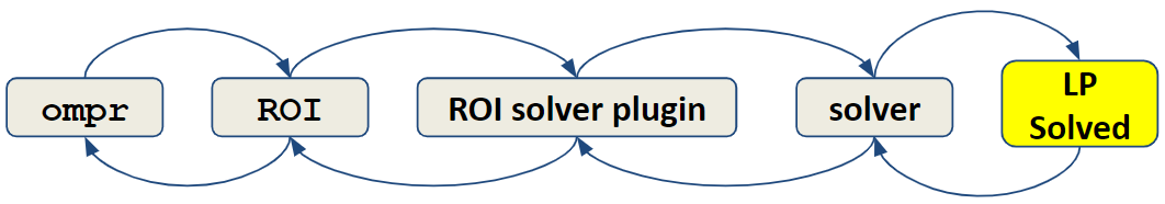
FIGURE 3.3: Relationship between ompr and solvers.
In general, the solver thinks of the problem in terms of a vector of coefficients for the objective function, C, a vector of right hand side constraint values, B, a matrix of data, A, and a vector of variables, x. The result is that any linear program can be thought of in a form to the right.
\[ \begin{split} \begin{aligned} \text{max } & C \cdot x \\ \text{s.t.: } & A \cdot x \leq B \\ & x \geq 0 \end{aligned} \end{split} \]
Let’s examine building our first two variable LP model in this way using the lpsolveAPI package.
\[ \begin{split} \begin{aligned} \text{Max } & 7\cdot Ants +12 \cdot Bats \\ \text{s.t.: } & 1\cdot Ants + 4 \cdot Bats \leq 800 \\ & 3\cdot Ants + 6 \cdot Bats \leq 900 \\ & 2\cdot Ants + 2 \cdot Bats \leq 480 \\ & 2\cdot Ants + 10 \cdot Bats \leq 1200 \\ & Ants, \; Bats \geq 0 \end{aligned} \end{split} \]
Now let’s implement the model the model using lpSolveAPI.
library(lpSolveAPI)
lps.model <- make.lp(0, 2) # Make empty 2 var model
add.constraint(lps.model, c(1,4), "<=", 800)
add.constraint(lps.model, c(3,6), "<=", 900)
add.constraint(lps.model, c(2,2), "<=", 480)
add.constraint(lps.model, c(2,10), "<=", 1200)
set.objfn(lps.model, c(-7,-12))
name.lp(lps.model, "Simple LP")
name.lp(lps.model)
## [1] "Simple LP"# plot.lpExtPtr(lps.model)
solve(lps.model)## [1] 0get.primal.solution(lps.model, orig=TRUE)## [1] 420 900 480 960 180 60While the graph may not be as elegant our earlier versions, it shows how the problem can be visualized.
Earlier in the chapter, we created data structures for the generalized version of the optimization model. Recall that earlier in this chapter we created a Resources matrix of the resources used by each product - this corresponds to our \(A\) matrix. We also created a single column matrix, Available, for the amount of each resource available which is our \(B\) vector. The Profit single row matrix serves as our \(C\) vector. The last item that we need to do is to specify a direction for each inequality.
We could rewrite our formulation then as the following.
\[ \begin{split} \begin{aligned} \text{max } & Profit \cdot x \\ \text{s.t. } & Resources \cdot x \leq Available \\ & x \geq 0 \end{aligned} \end{split} \]
The Rglpk package can then be accessed directly.
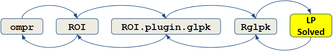
FIGURE 3.4: Relationship between ompr and Rglpk.
library (Rglpk) # Load Rglpk package## Loading required package: slam## Using the GLPK callable library version 4.47dir2<- c( "<=", "<=", "<=", "<=", "<=")
# Set direction of each inequality
res2 <- Rglpk_solve_LP(obj=Profit, # C vector
mat=Resources, # A matrix
dir=dir2, # Constraint Inequalities
Available, # B vector
max=TRUE) # False does minimization
# Uses default bounds on all variables:
# LB = 0, UB=infinity (just non-negativity)
# Defaults to continuous variablesNotice that calling the solver directly such as in this way using Rglpk does not require naming decision variables. A decision variable is created for each column of the matrix. Directly accessing the solver allows for all the same features that we use through ompr such as placing bounds on the variables, changing to a minimization objective function, and more such as advanced solving options. Other LP solving engines available in R such as RSymphony and lpSolve have similar syntax for solving. Let’s look at the results. As usual, we start by examining the status.
res2$status## [1] 0The status returned by Rglpk is zero. This may sound bad but the package’s help file indicates that returning a status value of zero means that no problems occurred and it found an optimal solution. We can then proceed to examine the objective function value.
res2$optimum## [1] 4800This objective function value may look familiar. Now let’s look at the solution in terms of optimal decision variable values.
res2$solution## [1] 240 0 0 0Most of these LP solving engines can also allow models to be built up incrementally as well by creating an empty model, then adding an objective function and adding constraints, bounds on variables as separate lines of R code.
While working with the solver directly has the benefit of avoiding ambiguities such as the difficulty of parsing solution status correctly, creating a single A matrix for optimization problems with multiple sets of decision variables and decision variables that may have 3 or more subscripts can be very tricky, hard to maintain, and even harder to debug. Also, the results require just as much or more care in unpacking as the solution variable values are returned as a single vector, x containing all the separate decision variables. Think of having three triple subscripted variables, u, v, and y with each subscript having 12 values. The resulting x vector will have \(3 \cdot 12^3=5184\) elements, each of which must always be considered in exactly the same order for each constraint or building of the A matrix.
At this point, it may be apparent that a chief benefit of ompr is that allows the modeler to deal with the model at a higher level and forces the computer to handle the detailed accounting translating the model into a lower level solvable structure and then translating the solution back into the original terms. These conversions are analogous to using a high level computer language versus a low level assembly code. A talented programmer can write a program in assembly code to do anything that could be done in a high level language but the cost in terms of time and effort is typically prohibitive.
The investment of time and effort to use a lower level, more direct access to the solver engine may be warranted when developing a package that does optimization. For example, packages for doing Data Envelopment Analysis require doing many linear programs. These are typically done using the lower level engines such as lpSolveAPI, Rglkp, lpSolveAPI, or other tools rather than ompr but the platform decision should be made carefully. A more indepth example of building optimization models using lower level access calls is in DEA Using R.
Since each low level solver may have different choices made in terms of the name or format of parameters to be passed for the LP as well as a different naming convention of elements being passed back, a translation layer has been developed, ROI which stands for the R Optimization Interface. There is the core ROI package and a specific ROI interface for each LP solver such as ROI.plugin.glpk. ROI can then be used to simplify switching between LP solvers. This is demonstrated in Chapter 8.
3.6 Exercises
Exercise 3.1 (Transportation) Four manufacturing plants are supplying material for distributors in four regions. The four supply plants are located in Chicago, Beaverton, Eugene, and Dallas. The four distributors are in PDX (Portland), SEA (Seattle), MSP (Minneapolis), and ATL (Atlanta). Each manufacturing plant has a maximum amount that they can produce. For example, Chicago can produce at most 500. Similarly, the PDX region can handle at most 700 units. The cost to transport from Dallas to MSP is three times as high as the cost from Dallas to Atlanta. The following table displays the transportation cost between all the cities.
| Node | PDX | SEA | MSP | ATL | Supply |
|---|---|---|---|---|---|
| Chicago | 20 | 21 | 8 | 12 | 500 |
| Beaverton | 6 | 7 | 18 | 24 | 500 |
| Eugene | 8 | 10 | 22 | 28 | 500 |
| Dallas | 16 | 26 | 15 | 5 | 600 |
| Capacity | 700 | 500 | 500 | 600 |
Formulate an explicit model for the above application that solves this transportation problem to find the lowest cost way of transporting as much as product as we can to distributors.
Hint: You might choose to define variables based on the first letter of source and destination so XCP is the amount to ship from Chicago to PDX.
Implement and solve the model using ompr.
Be sure to interpret and discuss the solution as to why it makes it sense.
Exercise 3.2 (Generalized Transportation Model) Formulate a generalized model for the above application that solves this transportation problem to find the lowest cost way of transporting as much product as we can to distributors.
Hint: Feel free to use my LaTeX formulation for the general transportation model and make change(s) to reflect your case.
Implement and solve the model using ompr. Be sure to discuss the solution as to why it makes sense.
Exercise 3.3 (Convert LP to Standard Form) Convert the three variable LP represented in Table 3.13 into standard form.
\[ \begin{split} \begin{aligned} \text{Max:} & \\ & Profit=20\cdot Ants+10\cdot Bats+16\cdot Cats \\ \text{S.t.} & \\ & 6\cdot Ants+3\cdot Bats+4\cdot Cats \leq 2000 \\ & 8\cdot Ants+4\cdot Bats+4\cdot Cats \leq 2000 \\ & 6\cdot Ants+3\cdot Bats+8\cdot Cats \leq 1440 \\ & 40\cdot Ants+20\cdot Bats+16\cdot Cats \leq 9600 \\ & Cats \leq 200 \\ & Ants, Bats, Cats \geq 0 \end{aligned} \end{split} \]
Exercise 3.4 (Solve Standard Form) Implement and solve the standard form of the LP using R. Be sure to interpret the solution and discuss how it compares to the solution from the original model.
Exercise 3.5 (Adding a Constraint) Add a new constraint to model in Exercise 3.4 such that number of Bats are double than the number of Ants. Be sure to interpret the solution and discuss how it compares to the solution from the original model.
Exercise 3.6 (Convert Generalized LP to Standard Form) Convert the following generalized production planning LP into standard form.
Hint: define a set of variables, \(s_j\) to reflect these changes and add it to the following formulation.
\[ \begin{split} \begin{aligned} \text{Maximize } & \sum_{i=1}^3 P_i x_i \\ \text{subject to } & \sum_{i=1}^3 R_{i,j}x_i \leq A_j \; \forall \; j\\ & x_i \geq 0 \; \forall \; i \end{aligned} \end{split} \]
Exercise 3.7 (Staff Scheduling) The need for nurses has increased rapidly during the Covid pandemic. Specific Hospital has determined their need for nurses throughout the day. They expect the following numbers of nurses to be needed over the typical 24 hour period. The nurses work eight hour shifts, starting at each 4 hour time period specified in the table.
hph_needs <- matrix (c(50, 140, 260, 140, 100, 80), ncol=1,
    dimnames = c(list(c("midnight - 4 AM",
                        "4 AM - 8 AM",
                        "8 AM - noon",
                        "noon - 4 PM",
                        "4 PM - 8 PM",
                        "8 PM - midnight")),
                 list(c("Required Nurses"))))
kbl (hph_needs, booktabs=T, caption="Staff Scheduling") |>
kableExtra::kable_styling(latex_options = "hold_position")| Required Nurses | |
|---|---|
| midnight - 4 AM | 50 |
| 4 AM - 8 AM | 140 |
| 8 AM - noon | 260 |
| noon - 4 PM | 140 |
| 4 PM - 8 PM | 100 |
| 8 PM - midnight | 80 |
- Create an appropriate optimization model to minimize the number of nurses needed to cover the requirements.
- Implement and solve the model in R.
- Discuss and explain your solution.
Exercise 3.8 (Reallocating personnel at Nikola) Due to the semiconductor shortage affecting the automotive industry, the production of vehicles has slowed down. The lack of a key control chip has brought the Engine shop of the manufacturing plant of automotive company Nikola to a complete halt. The company has decided to use the personnel from the Engine shop in other shops in the Press shop and the Paint shop, split equally. Also, it has decided to store the assembled vehicles in the plant until Engine Shop is functional again. The maximum capacity of the storage of cars is 10000. Current manpower and production information is as given in the table.
| Process Area | Alpha | Beta | Gamma | Theta | Available labor hours |
|---|---|---|---|---|---|
| Profit | $4000 | $3000 | $3600 | $5000 | |
| Press Shop | 1 | 3 | 2 | 2 | 600 |
| Weld Shop | 3 | 4 | 2 | 2 | 1200 |
| Paint Shop | 2 | 3 | 1 | 2 | 760 |
| Engine Shop | 3 | 5 | 2 | 4 | 700 |
| Assembly Shop | 2 | 0 | 2 | 0 | 1000 |
Make required change to the given table and Create an optimization model to find a production plan with max profit for all four car models - Alpha, Beta, Gamma, and Theta. Make sure to consider the max storage limit of 10000 cars.