Chapter 8 Goal Programming
8.1 Introduction
Up until this point, we assumed that there would be a single, clear objective function. Often we have more complex situations where there are multiple conflicting objectives. In our earlier production planning case, we might have additional objectives besides maximizing profit such as minimizing environmental waste or longer term strategic positioning. In the case of our capital budgeting problem, we can envision a range of additional considerations beyond simple expected net present value maximization. In the warehouse site selection problem from Chapter 7, we can envision other considerations such as political placement in certain states, being prepared for future varying growth levels in different regions, and other issues which could further influence a simple minimum cost solution.
8.2 Preemptive Goal Programming
Let’s begin with a simple example. Recall the example of multiple optima from Chapter 2. We had adjusted the characteristics of Cats so that there were multiple optima with different mixes of Ants and Cats. The LP solver found an initial solution that only produced Ants and we had to force the LP solver to find the Cats oriented production.
\[ \begin{split} \begin{aligned} \text{Max } & 7\cdot Ants +12 \cdot Bats +\textcolor{red}{14}\cdot Cats \\ \text{s.t.: } & 1\cdot Ants + 4 \cdot Bats +\textcolor{red}{2}\cdot Cats \leq 800 \\ & 3\cdot Ants + 6 \cdot Bats +\textcolor{red}{6}\cdot Cats \leq 900 \\ & 2\cdot Ants + 2 \cdot Bats +\textcolor{red}{4}\cdot Cats \leq 480 \\ & 2\cdot Ants + 10 \cdot Bats +\textcolor{red}{4}\cdot Cats \leq 1200 \\ & Ants, \; Bats, \; Cats \geq 0 \end{aligned} \end{split} \]
Let’s reframe this problem where the company’s primary goal is to maximize profit but the Cat product is more prestigious than the Ant product and emphasizing it will benefit the company in long term market positioning. The company doesn’t want to hurt profit but holding everything else equal, wants to then maximize Cat production.
The first step is to make the primary goal more direct. The objective function is now a fourth variable, Profit that is a direct function of the other three variables. The following formulation would then be considered the first phase.
\[ \begin{split} \begin{aligned} \text{Max } & \textcolor{red}{Profit}\\ \text{s.t.: } & \textcolor{red}{Profit=7\cdot Ants +12 \cdot Bats +14\cdot Cats} \\ & 1\cdot Ants + 4 \cdot Bats +2\cdot Cats \leq 800 \\ & 3\cdot Ants + 6 \cdot Bats +6\cdot Cats \leq 900 \\ & 2\cdot Ants + 2 \cdot Bats +4\cdot Cats \leq 480 \\ & 2\cdot Ants + 10 \cdot Bats +4\cdot Cats \leq 1200 \\ & Ants, \; Bats, \; Cats \geq 0 \end{aligned} \end{split} \]
The optimal objective function value from this LP is 1980 as shown in Chapter 2. Now we modify the above formulation to keep the Profit fixed at 1980 and maximize the production of Cats.
\[ \begin{split} \begin{aligned} \text{Max } & \textcolor{red}{Cats}\\ \text{s.t.: } & Profit=7\cdot Ants +12 \cdot Bats +14\cdot Cats \\ & 1\cdot Ants + 4 \cdot Bats +2\cdot Cats \leq 800 \\ & 3\cdot Ants + 6 \cdot Bats +6\cdot Cats \leq 900 \\ & 2\cdot Ants + 2 \cdot Bats +4\cdot Cats \leq 480 \\ & 2\cdot Ants + 10 \cdot Bats +4\cdot Cats \leq 1200 \\ & \textcolor{red}{Profit=1980}\\ & Ants, \; Bats, \; Cats \geq 0 \end{aligned} \end{split} \] Rather than directly stating the solution value of 1980, a more general approach would use the term, \(Profit^*\) to denote the optimal solution from the first Phase and the new Phase 2 constraint would then be \(Profit=Profit^*\). This would then give a revised solution that emphasizes Cat production in so far as it doesn’t detract from Profit. In other words, maximizing Profit preempts maximizing Cat production.
8.3 Policies for Houselessness
Let’s use an example that is a pressing issue for many cities - homelessness. Note that is often better characterized as houselesness and the term will be used interchangeably for the sake of this illustration.
The City of Bartland has a problem with houselessness. Two ideas have been proposed for dealing with the houselessness problem. The first option is to build new, government subsidized tiny homes for annual cost of \(\$10K\) which would serve one adult 90% of the time and a parent with a child 10% of the time. Another option is to create a rental subsidy program which costs \(\$25K\) per year per unit which typically serves a single adult (15%), two adults (20%), an adult with one child (30%), an adult with two children (20%), two adults with one child (10%), and two adults with two children (5%).
Bartland’s official Chief Economist has estimated that this subsidy program would tend to increase housing prices in a very tight housing market by an average of 0.001%. The Bartland City Council has \(\$1000K\) available to reappropriate from elsewhere in the budget and would like to find the best way to use this budget to help with the houselessness problem. Both programs require staff support - in particular 10% of a full time equivalent staff member to process paperwork, conduct visits, and other service related activities. There are seven staff members available to work on these activities.
Let’s summarize the data for two programs. Let’s focus on expected numbers of people served for each policy intervention.
| Per unit | Tiny Homes (H) | Rent Subsidy (R) |
|---|---|---|
| 1 adult | 90% | 15% |
| 1 adult, 1 child | 10% | 30% |
| 1 adult, 2 children | 0% | 20% |
| 2 adults | 0% | 20% |
| 2 adults, 1 child | 0% | 10% |
| 2 adults, 2 children | 0% | 5% |
| Expected children served | 0.1 | 0.9 |
| Expected adults served | 1.0 | 1.35 |
| Expected total people served | 1.1 | 2.25 |
| Cost per unit (\(\$K\)) | \(\$10\) | \(\$25\) |
| Staff support per unit | 0.1 | 0.1 |
One group on the city council wants to serve as many people (both children and adults) as possible while keeping under the total budget limit.
The second group feels that adults are responsible for their own situation but wants to save as many children from houselessness as possible within budget limits.
As usual, start by thinking of the decision variables. In this case, let’s define H to be number of tiny homes to be built and R to be the rental housing subsidies provided. Of course these should be non-negative variables. We could use integer variables or continuous variables.
Next let’s look at our constraints and formulate them in terms of the decision variables. We have two constraints. The first one for the budget is simply: \(10 \cdot H+ 25\cdot R \leq 1000\). The second is to ensure we have sufficient staff support, \(0.1 \cdot H+ 0.1\cdot R \leq 7\).
Now, let’s think about our objectives. The first group wants to serve as many people as possible so the objective function is \(\text {max } 1.1 \cdot H + 2.25 \cdot R\).
Similarly, since the second group is focused on children, their objective function is \[\text {max } 0.1\cdot H + 0.9\cdot R\].
Let’s put this all together in a formulation.
\[ \begin{split} \begin{aligned} \text{max } & 1.1 \cdot H + 2.25 \cdot R \\ \text{max } & 0.1 \cdot H + 0.9 \cdot R \\ \text{s.t. } & 10 \cdot H + 25 \cdot R \leq 1000 \\ & 0.1 \cdot H + 0.1 \cdot R \leq 7 \\ \ & H, \; R \; \in \{0, 1, 2, \ldots \} \end{aligned} \end{split} \]
Alas, linear programming models and the Simplex method only allows for a single objective function. Let’s start by solving from the perspective of the first group.
\[ \begin{split} \begin{aligned} \text{max } & 1.1 \cdot H + 2.25 \cdot R \\ \text{s.t. } & 10 \cdot H + 25 \cdot R \leq 1000 \\ & 0.1 \cdot H + 0.1 \cdot R \leq 7 \\ \ & H, \; R \; \in \{0, 1, 2, \ldots \} \end{aligned} \end{split} \]
Home1Model <- MIPModel() |>
 # Avoid name space conflicts by using a prefix of V
  add_variable(VH, type = "integer", lb = 0) |>
  add_variable(VR, type = "integer",lb = 0)  |>
  set_objective(1.1*VH + 2.25*VR,"max")      |>
  add_constraint(10*VH + 25*VR <= 1000)      |>
  add_constraint(0.1*VH + 0.1*VR <= 7)

res_Home1 <- solve_model(Home1Model,
                        with_ROI(solver = "glpk"))

H  <- get_solution (res_Home1 , VH)
R  <- get_solution (res_Home1 , VR)

sum_Home1           <- cbind(res_Home1$objective_value,H, R)
colnames(sum_Home1) <- c("Obj. Func. Val.", "H", "R")
rownames(sum_Home1) <- "Group 1: Max People"| Obj. Func. Val. | H | R | |
|---|---|---|---|
| Group 1: Max People | 100 | 50 | 20 |
Now, let’s examine the second group’s model that has an objective of maximizing the expected number of children served.
\[ \begin{split} \begin{aligned} \text{max } & 0.1 \cdot H + 0.9 \cdot R \\ \text{s.t. } & 10 \cdot H + 25 \cdot R \leq 1000 \\ & 0.1 \cdot H + 0.1 \cdot R \leq 7 \\ \ & H, \; R \; \in \{0, 1, 2, \ldots \} \end{aligned} \end{split} \]
Home2Model <- set_objective(Home1Model,
                            0.1*VH + 0.9*VR,"max")
  res_Home2 <- solve_model(Home2Model,
                        with_ROI(solver = "glpk"))

H  <- get_solution (res_Home2 , VH)
R  <- get_solution (res_Home2 , VR)

sum_Home2           <- cbind(res_Home2$objective_value,H, R)
colnames(sum_Home2) <- c("Obj. Func. Val.", "H", "R")
rownames(sum_Home2) <- "Group 2: Max Children"| Obj. Func. Val. | H | R | |
|---|---|---|---|
| Group 1: Max People | 100 | 50 | 20 |
| Group 2: Max Children | 36 | 0 | 40 |
So which group has the better model? The objective function value for group 1’s model is higher but it is in different units (people served) versus group 2’s model of children served.
Both group’s have admirable objectives. We can view this as a case of goal programming. By definition, we know that these are the best values that can be achieved in terms of that objective function. Let’s treat these optimal values as targets to strive for and measure the amount by which fail to achieve these targets. We’ll define target \(T_1 =\) 100 and \(T_2 =\) 36.
In order to do this, we need to use deviational variables. These are like slack variables from the standard form of linear programs. Since the deviations can only be one sided in this case, we only need to have deviations in one direction. We will define \(d_1\) as the deviation in goal 1 (Maximizing people served) and \(d_2\) as the deviation in goal 2 (Maximizing children served).
Let’s now create the modified formulation.
\[ \begin{split} \begin{aligned} \text{min } & d_1 + d_2 \\ \text{s.t. } & 10 \cdot H + 25 \cdot R \leq 1000 \\ & 0.1 \cdot H + 0.1 \cdot R \leq 7 \\ & 1.1 \cdot H + 2.25 \cdot R + d_1 = T_1 = 100 \\ & 0.1 \cdot H + 0.9 \cdot R + d_2 = T_2 = 36 \\ \ & H, \; R \; \in \{0, 1, 2, \ldots \} \\ \ & d_1, \; d_2 \geq 0 \end{aligned} \end{split} \]
| Obj. Func. Val. | H | R | d1 | d1% | d2 | d2% | |
|---|---|---|---|---|---|---|---|
| Min sum of deviations | 10 | 0 | 40 | 10 | 0.1 | 0 | 0 |
The deviation variables have different units though. One way to accommodate this would be to minimize the sum of percentages missed.
\[ \begin{split} \begin{aligned} \text{min } & \frac {d_1} {T_1} + \frac {d_2} {T_2} \\ \text{s.t. } & 10 \cdot H + 25 \cdot R \leq 1000 \\ & 0.1 \cdot H + 0.1 \cdot R \leq 7 \\ & 1.1 \cdot H + 2.25 \cdot R + d_1 = T_1 \\ & 0.1 \cdot H + 0.9 \cdot R + d_2 = T_2 \\ \ & H, \; R \; \in \{0, 1, 2, \ldots \} \\ \ & d_1, \; d_2 \geq 0 \end{aligned} \end{split} \]
## Status: optimal
## Objective value: 0.1| Obj. Func. Val. | H | R | d1 | d1% | d2 | d2% | |
|---|---|---|---|---|---|---|---|
| Min sum of deviation %s | 0.1 | 0 | 40 | 10 | 0.1 | 0 | 0 |
Another approach is to minimize the maximum deviation. This is often abbreviated as a minimax. This is essentially the same as the expression, “a chain is only as strong as its weakest link.” In Japan, there is an expression that the “the nail that sticks up, gets pounded down” and in China, “the tallest blade of grass gets cut down.” We can implement the same idea here by introducing a new variable, Q that must be at least as large as the largest miss. \[ \begin{split} \begin{aligned} \text{min } & Q \\ \text{s.t. } & 10 \cdot H + 25 \cdot R \leq 1000 \\ & 0.1 \cdot H + 0.1 \cdot R \leq 7 \\ & 1.1 \cdot H + 2.25 \cdot R + d_1 = T_1 \\ & 0.1 \cdot H + 0.9 \cdot R + d_2 = T_2 \\ & Q \geq \frac {d_1} {T_1} \\ & Q \geq \frac {d_2} {T_2} \\ \ & H, \; R \; \in \{0, 1, 2, \ldots \} \\ \ & d_1, \; d_2 \geq 0 \end{aligned} \end{split} \]
Let’s show the full R implementation of our minimax model.
Home5Model <- MIPModel() |>
 # To avoid name space conflicts, using a prefix of V
 #    for ompr variables.
  add_variable(VQ, type = "continuous")         |>
  add_variable(VH, type = "integer", lb = 0)    |>
  add_variable(VR, type = "integer",lb = 0)     |>
  add_variable(Vd1, type = "continuous",lb = 0) |>
  add_variable(Vd2, type = "continuous",lb = 0) |>
  set_objective(VQ ,"min")                      |>
  add_constraint(VQ>=Vd1/T1)                    |>
  add_constraint(VQ>=Vd2/T2)                    |>
  add_constraint(1.1*VH + 2.25*VR + Vd1 == T1)  |>
  add_constraint(0.1*VH + 0.9*VR + Vd2 == T2)   |>
  add_constraint(10*VH + 25*VR <= 1000)         |>
  add_constraint(0.1*VH + 0.1*VR <= 7)

res_Home5 <- solve_model(Home5Model,
                        with_ROI(solver = "glpk"))
res_Home5
## Status: optimal
## Objective value: 0.08H <- get_solution (res_Home5, VH)
R <- get_solution (res_Home5, VR)
d1 <- get_solution (res_Home5, Vd1)
d2 <- get_solution (res_Home5, Vd2)
sum_Home5 <- cbind(
res_Home5$objective_value, H, R,
d1, d1/T1, d2, d2/T2)
colnames(sum_Home5) <-
c("Obj. Func. Val.", "H", "R", "d1", "d1%", "d2", "d2%")
rownames(sum_Home5) <- "Minimax"| Obj. Func. Val. | H | R | d1 | d1% | d2 | d2% | |
|---|---|---|---|---|---|---|---|
| Min sum of deviations | 10.00 | 0 | 40 | 10 | 0.10 | 0.0 | 0.0000000 |
| Min sum of deviation %s | 0.10 | 0 | 40 | 10 | 0.10 | 0.0 | 0.0000000 |
| Minimax | 0.08 | 10 | 36 | 8 | 0.08 | 2.6 | 0.0722222 |
The minimax solution finds an alternative that is still Pareto optimal.
Careful readers may note that children are effectively double counted between the two objective functions when deviations are added.
This example can be expanded much further in the future with additional policy interventions, other stakeholders, and other characteristics, such as policies on drug addiction treatment, policing practices, and more. We did not factor in the Chief Economist’s impact on housing prices. We’ll leave these issues to future work.
8.4 Mass Mailings
Let’s take a look at another example. We have a mailing outreach campaign across the fifty states to do in the next eight weeks. You have \(C_s\) customers in each state. Since the statewide campaign needs to be coordinated, each state should be done in a single week but different states can be done in different weeks. You want to create a model to have the workload, in terms of numbers of customers, to be as balanced as possible across the eight weeks.
As an exercise, pause to think of how you would set this up.
What are your decision variables?
What are your constraints?
What is the objective function?
Try to give some thoughts as to how to set this up before moving on to seeing our formulation.
To provide some space before we discuss the formulation, let’s show the data. Rather than providing a data table that must be retyped, let’s use a dataset already available in R so you can simply load the state data. Note that you can grab the population in 1977 in terms of thousands.
data(state)
Customers <- state.x77[,1]
kbl (head (Customers), booktabs=T,
     caption="Number of Customers for First Six States.") |>
kable_styling(latex_options = "hold_position")| x | |
|---|---|
| Alabama | 3615 |
| Alaska | 365 |
| Arizona | 2212 |
| Arkansas | 2110 |
| California | 21198 |
| Colorado | 2541 |
8.4.1 Formulating the State Mailing Model
Presumably you have created your own formulation. If so, your model will likely differ from what follows in some ways such as naming conventions for variables or subscripts. That is fine. The process of trying to build a model is important.
Let’s start by defining our decision variables, \(x_{s,w}\) as a binary variable to indicate whether we are going to send a mailing to state s in week w.
Now, we need to ensure that every state is mailed to in one of the eight weeks. We simply need to add up the variable for each state’s decision to mail in week 1, 2, 3, …, up to 8. Mathematically, this would be \(\sum\limits_{w=1}^{8} x_{s,w} = 1, \; \forall \; s\).
It is useful to take a moment to reflect on why \(\sum\limits_{s=1}^{50} \sum\limits_{w=1}^{8} x_{s,w} = 50\) is not sufficient to ensure that all 50 states get mailed to during the eight week planning period.
Combined with the variable \(x_{s,w}\) being defined to be binary, this is sufficient to ensure that we have a feasible answer but not necessarily a well-balanced solution across the eight weeks.
We could easily calculate the amount of material to mail each as a function of \(x_s,w\) and \(C_s\). For week 1, it would be \(\sum\limits_{s=1}^{50} C_s \cdot x_{s,1}\) For week 2, it would be \(\sum\limits_{s=1}^{50} C_s \cdot x_{s,2}\), and so on. This could be generalized as \(\sum\limits_{s=1}^{50} C_s \cdot x_{s,w} \; \forall \; w\).
Creating a balanced schedule can be done in multiple ways. Let’s start by using the minimax approach discussed earlier. To do this, we add a new variable Q and constrain it to be at least as large as each week. Therefore, for week 1, \(Q \geq \sum\limits_{s=1}^{50} C_s \cdot x_{s,1}\) and for week 2, \(Q \geq \sum\limits_{s=1}^{50} C_s \cdot x_{s,2}\). Again, to generalize for all eight weeks, we could write \(Q \geq \sum\limits_{s=1}^{50} C_s \cdot x_{s,w} \; \forall \; w\).
we can then use our minimax objective function of simply minimizing Q.
We’ll summarize our formulation now.
\[ \begin{split} \begin{aligned} \text{min } & Q \\ \text{s.t. } & \sum\limits_{w=1}^{8} x_{s,w} = 1, \; \forall \; s \\ & Q \geq \sum\limits_{s=1}^{50} C_s \cdot x_{s,w} \; \forall \; w \\ \ & x_{s,w} \; \in \{0, 1 \} \; \forall \; s, \;w \\ \end{aligned} \end{split} \]
8.4.2 Implementing the State Mailing Model
Let’s now move on to implement this model in R.
States <- 50  # Options to shrink problem for testing
Weeks <- 8

Mail1 <- MIPModel()
     # 1 iff state s gets assigned to week w
Mail1 <- add_variable(Mail1, Vx[s, w],
                      s=1:States, w=1:Weeks, type="binary")

Mail1 <- add_variable(Mail1, VQ, type = "continuous")

Mail1 <- set_objective(Mail1, VQ, "min")

# every state  needs to be assigned to a week
Mail1 <- add_constraint(Mail1, sum_expr(Vx[s, w],
                          w=1:Weeks)==1, s=1:States)
Mail1 <- add_constraint(Mail1, VQ >=
                          sum_expr(Customers [s]*Vx[s, w],
                                   s=1:States), w = 1:Weeks)
Mail1
## Mixed integer linear optimization problem
## Variables:
## Continuous: 1
## Integer: 0
## Binary: 400
## Model sense: minimize
## Constraints: 58res_Mail1 <- solve_model(Mail1,
with_ROI(solver = "symphony",
verbosity=-1, gap_limit=1.5))res_Mail1## Status: infeasible
## Objective value: 26834Note that the the messages from Symphony indicate that the solution found was feasible while ompr interprets the status as infeasible. This is a bug that we have discussed earlier. Turning on an option for more messages from the solver such as verbose=TRUE for verbose=TRUE or verbosity=0 for symphony can give confirmation that the final status is not infeasible.
Another useful to thing to note is that solving this problem to optimality can take a long time despite having fewer binary variables than some of our earlier examples. Using glpk with verbose=FALSE means that the MIP is solved with no progress information displayed and makes it look like the solver is hung. Turning on more information (increasing the verbosity) helps explain that the Solver is working, it is just taking a while, on my computer I let it run 20 minutes without making further progress than a feasible solution it had found quickly.
In fact, I realized that the feasible solution found was very close to the best remaining branches so perhaps this solution was optimal but it was taking a very long time to prove that it was optimal. In any case, it is probably good enough. Often data may only be accurate to \(\pm5\%\) so spending extensive time trying to get significantly more accurate results is not very productive. This suggests setting stopping options such as a time limit, number of LPs, or a good enough setting. For this problem, I chose the latter option.
We solved this with a mixed integer programming problem gap limit of \(1.5\%\) meaning that while we have not proven this solution to be optimal, we do know that it is impossible to find a solution more than 1.5% better. From a branch and bound algorithm perspective, this means that while we have not searched down fully or pruned every branch, we know that no branch has the potential of being more than \(1.5\%\) better than the feasible solution that we have already found.
Now let’s move on to discussing the results. We will start with filtering out all the variables that have zero values so we can focus on the ones of interest - the states that are assigned to each week. Also, notice that a dplyr function was used to add state names to the data frame.
assigned1a <- res_Mail1 |>
 get_solution(Vx[s,w]) |>
 filter(value >.9) |>
 select (s,w)
rownames(assigned1a)<-c(names(Customers[assigned1a[,1]]))

kbl (head(assigned1a), booktabs=T,
     caption="Example of some states assigned to week 1") |>
kable_styling(latex_options = "hold_position")| s | w | |
|---|---|---|
| Indiana | 14 | 1 |
| Maryland | 20 | 1 |
| Minnesota | 23 | 1 |
| Nevada | 28 | 1 |
| North Carolina | 33 | 1 |
| South Carolina | 40 | 1 |
That is just for six states in the first week though.
assigned1b <- tibble::rownames_to_column(assigned1a)
table_results1<-c() # Prepare a new table of results
cols_list<-c()      # Prepare column list
weeksmail<-""

for (week_counter in 1:Weeks) {
  weeksmail1a<- assigned1b |>
  filter(w==week_counter) |>
  select(rowname)
  cols_list <- append(cols_list, paste0("Week ", week_counter))
  table_results1 <- append(table_results1,
                           paste(weeksmail1a$rowname,
                                 collapse = ", "))}

text_tbl <- data.frame(Weeks = cols_list,States = table_results1)kbl(text_tbl, booktabs=T,
caption="Display of States by Week") |>
kable_styling(latex_options = c("hold_position")) |>
column_spec(1, bold = T) %>%
column_spec(2, width = "30em")| Weeks | States |
|---|---|
| Week 1 | Indiana, Maryland, Minnesota, Nevada, North Carolina, South Carolina, Tennessee |
| Week 2 | Alabama, Arkansas, Delaware, Iowa, Montana, South Dakota, Texas, Washington |
| Week 3 | Alaska, Massachusetts, Missouri, Oregon, Pennsylvania, Utah, Vermont |
| Week 4 | Arizona, Hawaii, Idaho, Illinois, Kentucky, Maine, New Hampshire, West Virginia, Wisconsin |
| Week 5 | Colorado, Georgia, Ohio, Oklahoma, Rhode Island, Virginia |
| Week 6 | Florida, New York, Wyoming |
| Week 7 | California, Louisiana, New Mexico |
| Week 8 | Connecticut, Kansas, Michigan, Mississippi, Nebraska, New Jersey, North Dakota |
Since this is state level data, let’s look at a map of the schedule.
library (ggplot2)
library (maps)
mapx = data.frame(region=tolower(rownames(assigned1a)),
    week=assigned1a[,"w"],
    stringsAsFactors=F)

states_map <- map_data("state")
ggplot(mapx, aes(map_id = region)) +
    geom_map(aes(fill = week, colour = "white"),
             map = states_map) +
scale_fill_viridis_c(option = "C") +
expand_limits(x = states_map$long, y = states_map$lat)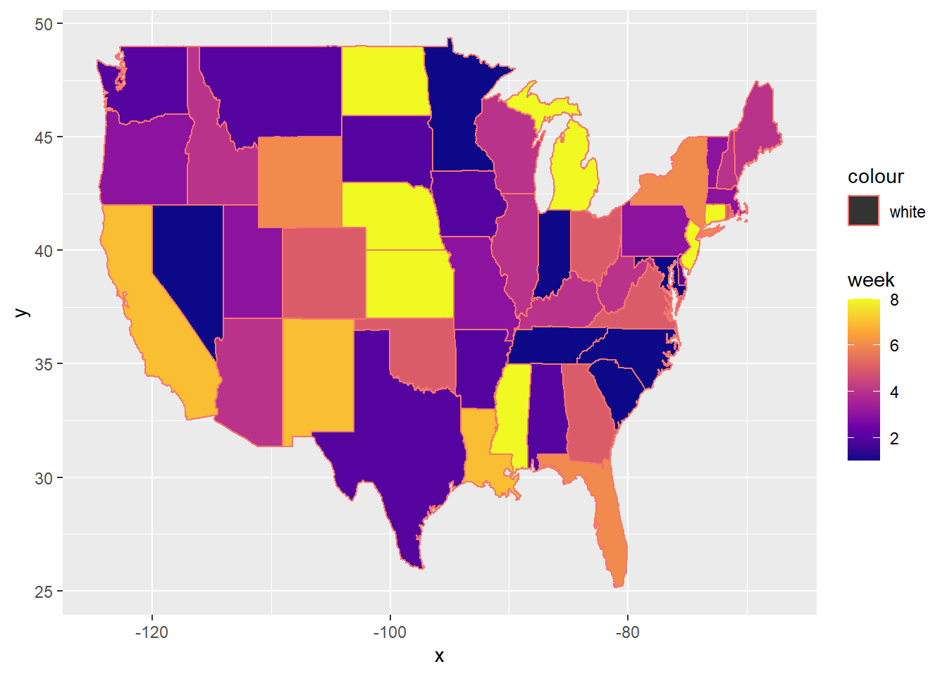
FIGURE 8.1: Map of Mailing Results
Note that this leaves off Alaska and Hawaii for visualization. For completeness, Alaska is in week 3 and Hawaii is in week 4.
8.4.3 Frontloading the Work
This formulation generates solutions that have high symmetry. Essentially it would be feasible and have the same objective function value if we simply swap any two weeks of assignments. For example, if we swap all of the states assigned to week 1 and week 2, it would still be feasible and have exactly the same objective function value. This would result in a high number of alternate optimal solutions. The numbering by week is essentially arbitrary since the weeks don’t make a difference.
When there exists a high degree of symmetry, it may be useful to implement one or more constraints to break the symmetry by differentiating between solutions. One approach to doing this is to require a particular ordering of weeks. For example, we could require that weeks get progressively lighter in terms of workload. In fact, this might be a managerial preference to ensure that if problems develop, there is some organizational slack later to deal with this.
\[ \begin{split} \begin{aligned} \sum\limits_{s=1}^{50} C_s \cdot x_{s,w-1} \geq \sum\limits_{s=1}^{50} C_s \cdot x_{s,w} , \; w \in \{2, \ldots ,8 \} \end{aligned} \end{split} \]
We could then extend our ompr model, Mail1 with the additional constraints.
Mail2 <- add_constraint(Mail1,
                        sum_expr(Customers [s]*Vx[s, w-1],
                              s=1:States) >=
               sum_expr(Customers [s]*Vx[s, w],
                              s=1:States),
               w = 2:Weeks)
While it might be thought that adding constraints limits the search space of possible solutions and might speed up solution, in this case it slows down solving speed tremendously. Despite having having less than half the binary variables of applications from Chapter 8 and the same number the earlier mail problem, this problem turns out to be most computationally demanding so far. The branch and bound process from symphony takes hours to solve.
kbl(as.matrix(table_results1[-1]), booktabs=T, caption=
      "Solution with Symmetry Breaking") |>
  kable_styling(latex_options = "hold_position")
The solving time using this modification to the LP changed tremendously. On an Intel i7 mobile CPU and R 4.1.1. the following results were obtained before terminating the solver after nearly four hours. Within 6 seconds it found a feasible solution as demonstrated by the Lower Bound of 26,540 but the upper bound of what could still be undiscovered was 29,602. This gives a possible suboptimality gap of 10.34%. Over the next half hour the Solver did not find a better solution (Lower Bound stays unchanged) but is able to reduce the Upper Bound. At this point I terminated the solver. There had been modest improvement in the search process in the first 30 minutes with two and a half million iterations (linear programming subproblems) but then no change for the three and half hours and almost six million more iterations.
| Seconds | Iterations | Lower Bound | Upper Bound | Gap (%) |
|---|---|---|---|---|
| 6 | 9,397 | 26540.12 | 29602.00 | 10.34 |
| 1291 | 2,015,431 | 26540.12 | 28940.00 | 8.24 |
| 1711 | 2,508,415 | 26540.12 | 28510.00 | 6.91 |
| 14311 | 8,391,692 | 26540.12 | 28510.00 | 6.91 |
This highlights that large or complex optimization problems may take extra effort and attention. Analysts can make judicious tradeoffs of potentially suboptimal results, solving time, and data accuracy. For our purpose, to speed up the solution time, you could do an early termination option such as setting the gap_limit to \(15\%\) by adding gap_limit=15. Setting an appropriate termination parameter based on gap, number of iterations, or time can be particularly helpful while developing a model. It also underscores that the benefits of implementing and testing algebraic models with smaller sized problems before expanding to the full sized problems. By separating the data from the model, we can easily just shrink or expand the problem without affecting the formulation or the implementation. In this case, we could shrink the problem by using fewer weeks and states by changing the upper limits (Weeks<-10; States<-10) used in the model, resulting in 30 binary variables instead of 400.
We could further modify the model to eliminate Q since the workload in week 1 would essentially be the heaviest workload (tallest nail.) This highlights that in optimization and particularly integer programming, there are often many different ways to implement models for the same application. This underscores the importance of clearly defining the elements of the formulation.
This application and model can be adjusted to fit a wide variety of other situations such as:
- Setting a maximum or minimum number of states per week
- Having a maximum and/or minimum number of customers to mail per week.
- Incorporating a secondary goal of finishing the mailing in as few weeks as possible.
- Applying this approach to other applications such as assigning customers to salespeople.
8.5 Exercises
Exercise 8.1 (Adjustments to Houselessness Policies) From the houselessness problem given in chapter, make changes as given below: First option is to build new, government subsidized tiny homes for annual cost of $15K which would serve one adult 85% of the time and a parent with a child 15% of the time. Another option is to create a rental subsidy program which costs $35K per year per unit which typically serves a single adult (15%), two adults (15%), an adult with one child (35%), an adult with two children (20%), two adults with one child (10%), and two adults with two children (5%).
Solve the problem and Discuss how the solution has changed.
Exercise 8.2 (Adjustments to Houselessness Policies) Create and justify your own third policy option to enhance the original exercise in the book. Describe the policy in the context of the application. Formulate, implement, and solve the revised version.
Does the revised solution match your expected result?
Exercise 8.3 (Extending State Mailing) The mailing by state example in chapter 8 is just another example of mixed integer programming.
- Write the optimization model using LaTeX to ensure that no week has more than 8 states assigned to the week.
- Write a constraint or set of constraints using LaTeX that would ensure state 3 is done before state 7.
- Write a constraint or set of constraints to ensure that state 9 and 24 are done in the same week.
- Given the minimax objective function, how do you think the above requirements will affect the solution in terms of an objective function and characteristics of managerial interest?
Exercise 8.4 (Experimenting with State Mailing) In the mailing by state example in chapter, there is a change discovered that Week 4 is going to be during a Holiday week and the Mailing Center will be closed for whole week. Make appropriate changes to the model in example presented in the chapter to reflect these changes.
- Write the optimization model using LaTeX to ensure that no week has more than 8 states assigned to the week.
- Write a constraint or set of constraints using LaTeX that would ensure state 4 is done before state 6.
- Write a constraint or set of constraints to ensure that state 5 and 9 are done in the same week.
- Write a constraint or set of constraints to ensure that the states of Oregon and California are done before holiday week.
- After solving above, compare the results with exercise 8.1 and discuss.